Hashing - Collisions

HashMap works

1) First of all, key object is checked for null. If key is null, value is stored in table[0] position. Because hash code for null is always 0.

2) Then on next step, a hash value is calculated using key’s hash code by calling its hashCode() method. This hash value is used to calculate index in array for storing Entry object. JDK designers well assumed that there might be some poorly written hashCode() functions that can return very high or low hash code value. To solve this issue, they introduced another hash() function, and passed the object’s hash code to this hash() function to bring hash value in range of array index size.

3) Now indexFor(hash, table.length) function is called to calculate exact index position for storing the Entry object.

4) Here comes the main part. Now, as we know that two unequal objects can have same hash code value, how two different objects will be stored in same array location [called bucket].
Answer is LinkedList. If you remember, Entry class had an attribute “next”. This attribute always points to next object in chain. This is exactly the behavior of LinkedList.

Collisions

What happens, if hash function returns the same hash value for different keys? It yields an effect, called collision. Collisions are practically unavoidable and should be considered when one implements hash table. Due to collisions, keys are also stored in the table, so one can distinguish between key-value pairs having the same hash. There are various ways of collision resolution. Basically, there are two different strategies:

• Closed addressing (open hashing). Each slot of the hash table contains a link to another data structure (i.e. linked list), which stores key-value pairs with the same hash. When collision occures, this data structure is searched for key-value pair, which matches the key.
• Open addressing (closed hashing). Each slot actually contains a key-value pair. When collision occurs, open addressing algorithm calculates another location (i.e. next one) to locate a free slot. Hash tables, based on open addressing strategy experience drastic performance decrease, when table is tightly filled (load factor is 0.7 or more).

Open Addressing

Like Closed addressing, open addressing is a method for handling collisions. In Open Addressing, all elements are stored in the hash table itself. So at any point, size of table must be greater than or equal to total number of keys (Note that we can increase table size by copying old data if needed).

Insert(k): Keep probing until an empty slot is found. Once an empty slot is found, insert k.

Search(k): Keep probing until slot’s key doesn’t become equal to k or an empty slot is reached.

Delete(k): Delete operation is interesting. If we simply delete a key, then search may fail. So slots of deleted keys are marked specially as “deleted”.
Insert can insert an item in a deleted slot, but search doesn’t stop at a deleted slot.

Open Addressing is done following ways:

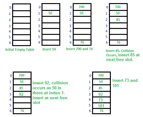
a) Linear Probing: In linear probing, we linearly probe for next slot. For example, typical gap between two probes is 1 as taken in below example also.
let hash(x) be the slot index computed using hash function and S be the table size

If slot hash(x) % S is full, then we try (hash(x) + 1) % S
If (hash(x) + 1) % S is also full, then we try (hash(x) + 2) % S
If (hash(x) + 2) % S is also full, then we try (hash(x) + 3) % S 
..................................................
..................................................

Let us consider a simple hash function as “key mod 7” and sequence of keys as 50, 700, 76, 85, 92, 73, 101.

Clustering: The main problem with linear probing is clustering, many consecutive elements form groups and it starts taking time to find a free slot or to search an element.

b) Quadratic Probing We look for i2‘th slot in i’th iteration.

let hash(x) be the slot index computed using hash function.  
If slot hash(x) % S is full, then we try (hash(x) + 1*1) % S
If (hash(x) + 1*1) % S is also full, then we try (hash(x) + 2*2) % S
If (hash(x) + 2*2) % S is also full, then we try (hash(x) + 3*3) % S
..................................................
..................................................

c) Double Hashing We use another hash function hash2(x) and look for i*hash2(x) slot in i’th rotation.

let hash(x) be the slot index computed using hash function.  
If slot hash(x) % S is full, then we try (hash(x) + 1*hash2(x)) % S
If (hash(x) + 1*hash2(x)) % S is also full, then we try (hash(x) + 2*hash2(x)) % S
If (hash(x) + 2*hash2(x)) % S is also full, then we try (hash(x) + 3*hash2(x)) % S
..................................................
..................................................

Comparison of above three:
Linear probing has the best cache performance, but suffers from clustering. One more advantage of Linear probing is easy to compute.

Quadratic probing lies between the two in terms of cache performance and clustering.

Double hashing has poor cache performance but no clustering. Double hashing requires more computation time as two hash functions need to be computed.

Open Addressing vs. Closed addressing
Advantages of Chaining:
1) Chaining is Simpler to implement.
2) In chaining, Hash table never fills up, we can always add more elements to chain. In open addressing, table may become full.
3) Chaining is Less sensitive to the hash function or load factors.
4) Chaining is mostly used when it is unknown how many and how frequently keys may be inserted or deleted.
5) Open addressing requires extra care for to avoid clustering and load factor.

Advantages of Open Addressing
1) Cache performance of chaining is not good as keys are stored using linked list. Open addressing provides better cache performance as everything is stored in same table.
2) Wastage of Space (Some Parts of hash table in chaining are never used). In Open addressing, a slot can be used even if an input doesn’t map to it.
3) Chaining uses extra space for links.

Performance of Open Addressing:
Like Chaining, performance of hashing can be evaluated under the assumption that each key is equally likely to be hashed to any slot of table (simple uniform hashing)
 m = Number of slots in hash table
 n = Number of keys to be inserted in has table
 
 Load factor α = n/m  ( < 1 )

 Expected time to search/insert/delete < 1/(1 - α) 

 So Search, Insert and Delete take (1/(1 - α)) time

Closed Addressing:
The idea is to make each cell of hash table point to a linked list of records that have same hash function value.

Let us consider a simple hash function as “key mod 7” and sequence of keys as 50, 700, 76, 85, 92, 73, 101.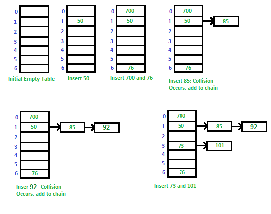

Advantages:
1) Simple to implement.
2) Hash table never fills up, we can always add more elements to chain.
3) Less sensitive to the hash function or load factors.
4) It is mostly used when it is unknown how many and how frequently keys may be inserted or deleted.

Disadvantages:
1) Cache performance of chaining is not good as keys are stored using linked list. Open addressing provides better cache performance as everything is stored in same table.
2) Wastage of Space (Some Parts of hash table are never used)
3) If the chain becomes long, then search time can become O(n) in worst case.
4) Uses extra space for links.

Performance of Chaining:
Performance of hashing can be evaluated under the assumption that each key is equally likely to be hashed to any slot of table (simple uniform hashing).
 m = Number of slots in hash table
 n = Number of keys to be inserted in has table
 
 Load factor α = n/m 
  
 Expected time to search = O(1 + α)
 
 Expected time to insert/delete = O(1 + α)

 Time complexity of search insert and delete is 
 O(1) if  α is O(1)